High-Dimensional Statistics: Concentration Inequalities

Introduction

In a variety of settings, one often would like to establish statistical guarantees for the performance of machine learning algorithms. These guarantees help us understand how fast an algorithm converges in expectation and how many samples we may need. One powerful tool for obtaining such guarantees is the use of concentration inequalities. Concentration inequalities provide bounds on the probability that a random variable deviates from some central value, such as its mean. They are crucial in theoretical machine learning for deriving bounds on the performance of estimators, classifiers, and other statistical models. By leveraging these inequalities, researchers can rigorously quantify the reliability and accuracy of their algorithms, even when dealing with complex, high-dimensional data. This article explores various concentration inequalities and their applications in machine learning literature, particularly analyzing convergence rates in lasso.

Classical Bounds

Many of you will be familiar with Markov's and Chebyshev's Inequalities. These are common (yet crude) bounds for controlling tail probabilities $\mathbb{P}(X \geq t)$. You will often hear that Chebyshev's inequality is a much sharper bound (but requires a little bit more information) compared to Markov. This is because as we get control of higher-order moments, this leads to correspondingly sharper bounds on tail probabilities. This ranges from Markov (where we only need first moment information) to inequalities like Chernoff (which require the existence of a moment generating function (MGF)). In the context of this section, assume that we have a random variable $X \sim \mathbb{P}_{X}$ sampled from a probability distribution $\mathbb{P}_X$ defined on a probability space $\left(\Omega, \Sigma, P\right)$

Markov's Inequality

Let's first talk about the most basic concentration inequality. Suppose we have a non-negative random variable $X$ with finite mean. Then,

Chebyshev's Inequality

As we discussed before, we can try to get tighter tail probabilities by controlling higher-order moments. Suppose that we have a random variable $X$ with finite variance. Furthermore, let us denote $\mu = \mathbb{E} \left[ X \right]$. Then,

Chernoff Bound

In Markov and Chebyshev's inequality, we simply assumed that our random variable $X$ had finite first and second-order moments. Now, suppose that we have a random variable $X$ with a defined moment-generating function in a neighborhood of $0$, meaning that there exists some $b > 0$ such that the function $\phi(\lambda) = \mathbb{E} \left[ e^{\lambda(X - \mu)} \right]$ exists for all $\lambda \leq |b|$. Then, for any $\lambda \in [0, b]$

Simple Illustration of The Power of Bounding Higher Moments

One may be wondering how drastic the difference is in bounding higher moments. Let's do an example. Suppose that $X \sim \mathrm{Binomial}(n, p)$. Below, we see how the Markov, Chebyshev, and Chernoff bound varies with the actual tail probability as $t$ varies. We see that Markov is indeed a crude bound to the true tail probability while Chebyshev and Chernoff do a much better job of approximating the tail probability. In fact, notice that Chernoff converges to the true tail probability much faster compared to Chebyshev.

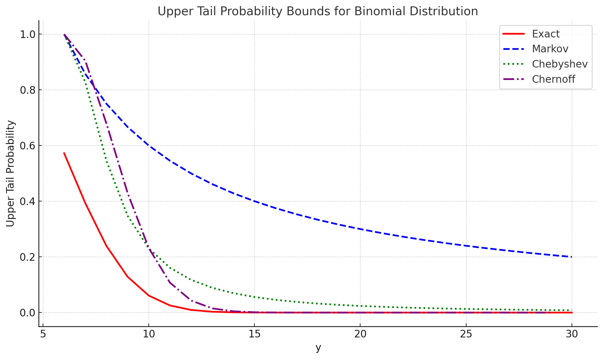
How does this relate to moments? Well, notice that Chernoff's bound is simply the Legendre-Fenchel transform of the $\log$ of the moment-generating function which is also called the cumulant-generating function. Now, if we do the calculations of the cumulants for the Binomial distribution (I will leave this as an exercise), we will see that the CGF is essentially giving us information for the first, second, and third order-moments about the mean. Simply put, having the MGF exist and thus the CGF gives us more information about higher-order moments compared to bounds like Markov and Chebyshev which use first and second order moment information respectively. That is not to say that Markov and Chebyshev bounds cannot be tight. There are examples where Markov and Chebyshev are tight (think about how you can construct an example of this). In most cases, it is true that Chernoff will be tigher simply since it has more information about higher-order moments encoded in its construction. This illustrates the power of bounding higher moments!

Sub-Gaussian Variables and Hoeffding Bounds

As we could see from the Chernoff bound, we require the existence of the MGF of the random variable in the neighborhood of $0$. As one would assume, the Chernoff bound naturally depends on the growth rate of the MGF. Accordingly, we can classify random variables by the growth rate of their MGFs. The simplest behavior is known as sub-Gaussian. We define this as follows

Definition (Sub-Gaussian Random Variables): A random variable $X$ with mean $\mu = \mathbb{E}[X]$ is called sub-Gaussian if there exists a positive number $\sigma$ such that

Why is this called sub-Gaussian? A quick derivation (again I will leave this as an exercise) shows that for $X \sim \mathcal{N}(\mu, \sigma^2)$ has an MGF of $M_{X}(\lambda) = e^{\lambda \mu + \lambda^2 \sigma^2 / 2}$. Sub-Gaussian random variables are powerful since they allow us to categorize distributions that are not Gaussian as having tails that decay at-least as fast as Gaussian distributions. Given that we know many important and useful properties of Gaussian distributions, it is easy to see why these are important. Let's look at some random variables that are not Gaussian but are sub-Gaussian. These examples come from Wainwright's High-Dimensional Statistics book [1], a book I would highly recommend if you want to learn more about high-dimensional statistics.

Example: Let $\varepsilon \sim \mathrm{Unif} \lbrace -1, 1 \rbrace$. This is known as a Rademacher random variable which takes on values of either $-1$ or $1$, each with probability $1/2$. Then, using the Taylor series expansion for the exponential, we see that

where the inequality follows since $2k! \geq k! \ 2^k$ (Why does this hold? Try expanding $2k!$ and see what you notice). We see that $\varepsilon \sim \mathrm{SG}(1)$

Example: Let $X$ be zero-mean, and let $\mathrm{supp} X \subseteq [a, b]$. Then, let $X^{\prime} \sim \mathbb{P}_{X}$. For any $\lambda \in \mathbb{R}$, we have that

Here, we will apply a clever trick called symmetrization. Let $\varepsilon \sim \mathrm{Unif} \lbrace -1, 1 \rbrace$. Then, notice that distributionally, $\varepsilon (X - X^{\prime}) \stackrel{d}{=} X - X^{\prime}$ because if $\varepsilon = -1$, then we already know that $X^{\prime} - X \stackrel{d}{=} X - X^{\prime}$ and the $\varepsilon = 1$ case is trivial to see why it is equivalent. We will also apply that we learned above about $\varepsilon \sim \mathrm{SG}(1)$. Applying these, we get

Since we have that $\mathrm{supp} X \in [a, b]$, the deviation $|X - X^{\prime}|$ is atmost $b-a$. Thus, we can conclude that

This implies that $X \sim \mathrm{SG}(b-a)$. We will use this result to prove another concentration inequality called the Hoeffding bound.

Hoeffding Bound

Suppose that we have random variables $X_{i} \stackrel{i.i.d}{\sim} \mathrm{SG}(\sigma_{i})$ with mean $\mu_{i}$. Then, for all $t \geq 0$, we have

We could have also stated the Hoeffding bound in terms of bounded random variables. Suppose $\mathrm{supp} X_{i} \subseteq [a, b]$ with mean $\mu _{i}$. Then, from the example above, we know that $X_{i} \stackrel{i.i.d}{\sim} \mathrm{SG}(b-a)$. Thus, it can be stated that

Sub-Gaussian Maximal Inequalities

We can use this identifying property of Sub-Gaussian random variables to prove many useful inequalities. One which will become important in our discussions is the sub-Gaussian maximal inequalities. That is, suppose $X_{i} {\sim} \mathrm{SG}(\sigma)$ with mean $0$. Notice that we have no independence assumptions. Then,

We can use this result to prove other simple results such as $\mathbb{E} \left[ \mathrm{max}_{i=1, ..., n} |X_{i}| \right] \leq 2\sqrt{ \sigma^{2} \log{n}}$ or showing that $\mathbb{P} \left( \mathrm{max}_{i=1, ..., n} X_{i} \geq \sigma \sqrt{2 \left( \log{n} + t \right) } \right) \leq e^{-t}$ for any $t > 0$ (I leave these as exercises). We can use these results to prove what are sometimes called the "slow" rates and "oracle inequality" for Lasso regularization.

Quick Review of Lasso, "Slow Rates", and the "Oracle Inequality"

The details that follow largely come from Statistics 241B: Statistical Learning Theory, a course that I took at UC Berkeley while I was an undergraduate. It was taught by Ryan Tibshirani who was a great instructor and mentor for me, and I highly recommend you to check out his Statistical Learning course. All the course notes and materials are readily available on his website [3]. Now, let's do a quick recap on least-squares.

Suppose we have $n$ observations $ \lbrace \left( x_{i}, y_{i} \right) \rbrace_{i=1}^{n}$ where each $x_{i} \in \mathbb{R}^{d}$ is a feature vector and $y_{i}$ is the associated response value. Horizontally stacking these features creates a matrix that we can denote $X \in \mathbb{R}^{n \times d}$. Likewise, vertically stacking the response values creates a vector $Y \in \mathbb{R}^{n}$. Recall that the least-squares coefficients are determined by solving the following optimization problem

By the rank-nullity theorem, if $n > > d$, then $\mathrm{rank}\left( X \right) \leq d$. Thus, $\mathrm{nullity} \left(X \right) \geq 0$. If $\mathrm{rank}\left( X \right) = d$, then of course we get that $\mathrm{nullity} \left( X \right) = 0$. Thus, there is a unique solution for least-squares which is

Then, the in-sample predictions (also known as the fitted-values) are simply

This is equivalenly $X\beta = \Pi_{\mathrm{Col} \left( X \right)}Y$ where $\Pi$ is the projection operator. Now, to justify some of the reasons why we use Lasso, we need to investigate the in-sample and out-of-sample risk of least-squares regression. Assume that $ \lbrace \left( x_{i}, y_{i} \right) \rbrace_{i=1}^{n}$ are i.i.d such that $X^{\top}X$ is almost surely invertible. Also, let

where $\varepsilon_{i}$ has mean $0$ and variance $\sigma^{2}$ and $x_{i}$ is independent of $\varepsilon_{i}$. Then, the in-sample risk is simply the bias-variance decomposition with $X$ being fixed. Since $\mathbb{E} \left[ X \hat{\beta} | X \right] = X\beta_{0}$, we see that least-squares has zero bias in the in-sample case. Thus, the risk is purely determined by the variance which we can compute to get

We do a similar thing for calculating the out-of-sample risk. In this case, we assume that $X$ is random and that $X$ is independent of $\varepsilon$ with $\left( x_{0}, y_{0} \right)$ being drawn i.i.d from the same linear model. Then, we see that

we see that least-squares has zero bias in the out-of-sample case. Again, the risk is purely determined by the variance which we can compute to get

Thus, we get that the out-of-sample risk is

Clearly, we see that the in-sample and out-of-sample risk increases greatly if $d > n$. Furthermore, we cannot even guarantee that the solution to least-squares is unique since by the rank-nullity theorem, $\mathrm{nullity} \left(X \right) \geq d - n$ so any vector of the form

is a solution to least-squares. Notice that we used the pseudoinverse of $X^{\top}X$ instead since if the $\mathrm{nullity} \left(X \right) \geq d - n$ and $\mathrm{rank} \left( X \right) = \mathrm{rank} \left( X^{\top}X \right)$, we clearly see that $X^{\top}X$ is rank-deficient so it will not have an inverse. Now, we define the least absolute selection and shrinkage operator or Lasso as

As we increase the tuning parameter $\lambda$, we typically get sparser solutions since as $\lambda \rightarrow \infty$, the only way to minimize the objective is to push the coefficients of $\beta \rightarrow 0$. As a result, we also care less about the least-squares loss. Now, why do we care about sparsity? There are two reasons Lasso is desirable. The first reason is that it corresponds to performing variable selection on the fitted linear model which allows us to understand which features are important and increase the interpretability of our model. The second reason is that it often will predict better in situations where the true regression function is well-approximated by a sparse linear model. As a data-scientist, you often want to find the best subset of features that decreases out-of-sample risk so you may use methods like forward selection or backward selection. It turns out that Lasso is closely related to best subset selection and thus Lasso is usually a pretty decent place to start in regards to variable selection. There is a lot of interesting theory and properties of Lasso but we shall move onto talking about Lasso's "slow" rates and "oracle inequality" for prediction risk.

Lasso "Slow" Rates

In this setting, we will assume a linear model $Y = X\beta_{0} + \varepsilon$ where $\varepsilon \sim \mathrm{SG}\left( \sigma \right)$ with mean $0$. We will take $X \in \mathbb{R}^{n \times d}$ to be fixed and assume that $\mathrm{max}_{j = 1, ..., d} ||X_{j}||_{2} \leq \sqrt{n}$. Let $\hat{\beta} = \mathrm{argmin}_{\beta} \frac{1}{2} ||Y - X\beta||_{2}^{2} + \lambda ||\beta||_{1}$. Then, for any $\beta \in \mathbb{R}^{d}$,

Thus, we can rearrange this to get

Adding and subtracting $X\beta$ on both sides yields

Since this holds for any $\beta \in \mathbb{R}^{d}$, we take $\beta = \beta_{0}$. Notice that $Y - X\beta = \varepsilon$ so we get

Notice that by Hölder's Inequality, we get

Using this inequality coupled with the triangle inequality and taking $\lambda \geq 2||X^{\top}\varepsilon||_{\infty}$, we get

Now, notice the following. $X^{\top}\varepsilon$ has mean $0$ and has variance proxy $\mathrm{max}_{j = 1, ..., d} ||X_{j}||_{2}^{2} \sigma^{2} \leq n \sigma^{2}$ (this is a simple exercise to show). Thus, we have that $X^{\top}\varepsilon \sim \mathrm{SG} \left( n \sigma^{2} \right)$. Using the sub-Gaussian maximal inequality we derived above (in particular the probability bound), we have that

If we take $\lambda = \sigma \sqrt{2n \left( \log{\left( 2d \right)} + u \right)}$, we can make a probabilistic argument of $\lambda \geq 2||X^{\top}\varepsilon||_{\infty}$. Thus, we conclude by saying that

with probability at least $1 - e^{-u}$. This is what we call the "slow" rate of Lasso and it tells us that the in-sample risk scales as $\mathcal{O}\left( ||\beta_{0}||_{1} \sqrt{\frac{\log{\left(d \right)}}{n}} \right)$. Something to note is that the constrained form of Lasso and the penalized form have the same "slow" rate. This is simple to prove. Simply repeat the steps 1-3 without the penalty term of the proof above and take the threshold to be $||\beta_{0} ||_{1}$. The steps after that are the same using the probabilistic argument.

Lasso "Oracle Inequality"

Suppose that we do not want to assume a linear model for the underlying regression. Instead, let us assume that $Y = f_{0} (X) + \varepsilon$ for some function $f_{0}: \mathbb{R}^{d} \rightarrow \mathbb{R}$. We will use the constrained form of Lasso. Then, for any $\overline{\beta} \in \mathbb{R}^{d}$ with $||\overline{\beta}||_{1} \leq t$, we get

Using the identity $||a||_{2}^{2} + ||b||_{2}^{2} - ||a - b||_{2}^{2} = 2 \langle a, b \rangle$ on the first term, we get

Cancelling and rearranging terms, we get

with probability at least $1 - e^{-u}$. Since this holds for all estimators $\overline{\beta}$ where $||\overline{\beta}||_{1} \leq t$, we can say

This is called the "oracle inequality" for the constrained lasso estimator. What is says in terms of in-sample risk is that the lasso predictor is expected to perform as well as the best $l_{1}$ sparse predictor to $f_{0}$. With a few simple tools from concentration inequalities, we were able to prove something as fundamental as in-sample estimation rates of the Lasso.

@article{sahu2024concentrationinequalities,
  title   = "High-Dimensional Statistics: Concentration Inequalities.",
  author  = "Sahu, Sharan",
  journal = "sharansahu.com",
  year    = "2024",
  month   = "Jul",
  url     = "https://sharansahu.com/posts/post1/concentration-inequalities.html/"
}

References

- Wainwright, High-Dimensional Statistics: A Non-Asymptotic Viewpoint. Chapter 1.
- Tibshirani, R. (2023). Stat 241B: Lasso and sparse regression models. University of California, Berkeley. https://www.stat.berkeley.edu/~ryantibs/statlearn-s23/lectures/lasso.pdf.
- Trevor Hastie, Robert Tibshirani, and Jerome Friedman. The Elements of Statistical Learning: Data Mining, Inference and Prediction. Springer, 2009. Second edition.